Introduction

The mbte-package aims to generalize the workflow regarding the exploratory data analysis of time-dependent data. The approach is based on the Managing many models- talk by Hadley Wickham.

Example workflow

First, the required packages are loaded:

library(dplyr)
library(tidyr)
library(purrr)
library(ggplot2)
library(mbte)

The raw_signals-dataset is used for this demonstration.

data("raw_signals")
raw_signals
#> # A tibble: 4,200 x 3
#>        t mv    value
#>    <int> <chr> <dbl>
#>  1     1 mv1       0
#>  2     2 mv1       0
#>  3     3 mv1       0
#>  4     4 mv1       0
#>  5     5 mv1       0
#>  6     6 mv1       0
#>  7     7 mv1       0
#>  8     8 mv1       0
#>  9     9 mv1       0
#> 10    10 mv1       0
#> # … with 4,190 more rows

The raw_signals-dataset is an exclusively fictional dataset, which consists of 3 columns:

t: The time-column indicating when the measurement was made.
mv: The measurement-variable - the measured parameter.
value: The intensity of the measurement variable.

The goal is to estimate, if trends of different measured parameters are present.

Creation of the main datastructure

Because raw_signals is a tibble, new_tbl_mbte() is used to convert it to a tbl_mbte (the main datastructure of the mbte-package). new_tbl_mbte() takes tibbles as first argument or objects, that can be converted to tibbles via tibble::as_tibble(). Additionally, column names for the time and the value-columns are passed too.

# pass as strings
raw_signals <- new_tbl_mbte(raw_signals, time = "t", value = "value")

It would be possible to rely on quotation too:

raw_signals <- new_tbl_mbte(raw_signals, time = t, value = value)

Nesting of signals

In the following step, the time- and value- columns get combined into a new list-column, which is consisting of tibbles (signal-column). A parameter for grouping must be specified. Since the goal is to find out which measurement- variables contain trends, the mv-column is used for grouping (contains the names of the measured parameters).

nested <- mbte_nest_signals(raw_signals, "mv")
nested
#> # A tibble: 42 x 2
#>    mv    signal            
#>    <chr> <list>            
#>  1 mv1   <tibble [100 × 2]>
#>  2 mv2   <tibble [100 × 2]>
#>  3 mv3   <tibble [100 × 2]>
#>  4 mv4   <tibble [100 × 2]>
#>  5 mv5   <tibble [100 × 2]>
#>  6 mv6   <tibble [100 × 2]>
#>  7 mv7   <tibble [100 × 2]>
#>  8 mv8   <tibble [100 × 2]>
#>  9 mv9   <tibble [100 × 2]>
#> 10 mv10  <tibble [100 × 2]>
#> # … with 32 more rows

Also here, the passed variables get quoted. Therefore, the following call is equivalent to the one above.

nested <- mbte_nest_signals(raw_signals, mv)

Each subtibble contains the complete signal for the chosen grouping:

nested$signal[[5]] # print example signal-subtibble
#> # A tibble: 100 x 2
#>        t value
#>    <int> <dbl>
#>  1     1  0   
#>  2     2  0   
#>  3     3  0   
#>  4     4  0   
#>  5     5  0   
#>  6     6  0   
#>  7     7  0   
#>  8     8  0   
#>  9     9  4.40
#> 10    10  3.02
#> # … with 90 more rows

Subsignal extraction

For some specific usecases, it may be required, that the extracted signal- table gets split into subsignals. This may be necessary if only nonzero signal-values are analyzed. The following plots show the unextracted signals. The parts highlighted in blue will be kept (extracted subsignals). The dashed red line indicates \(y = 0\).

#> [[1]]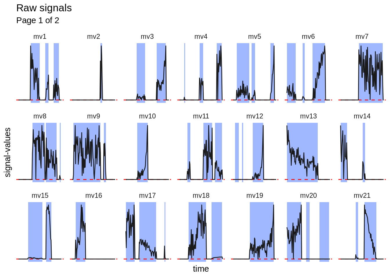

#> 
#> [[2]]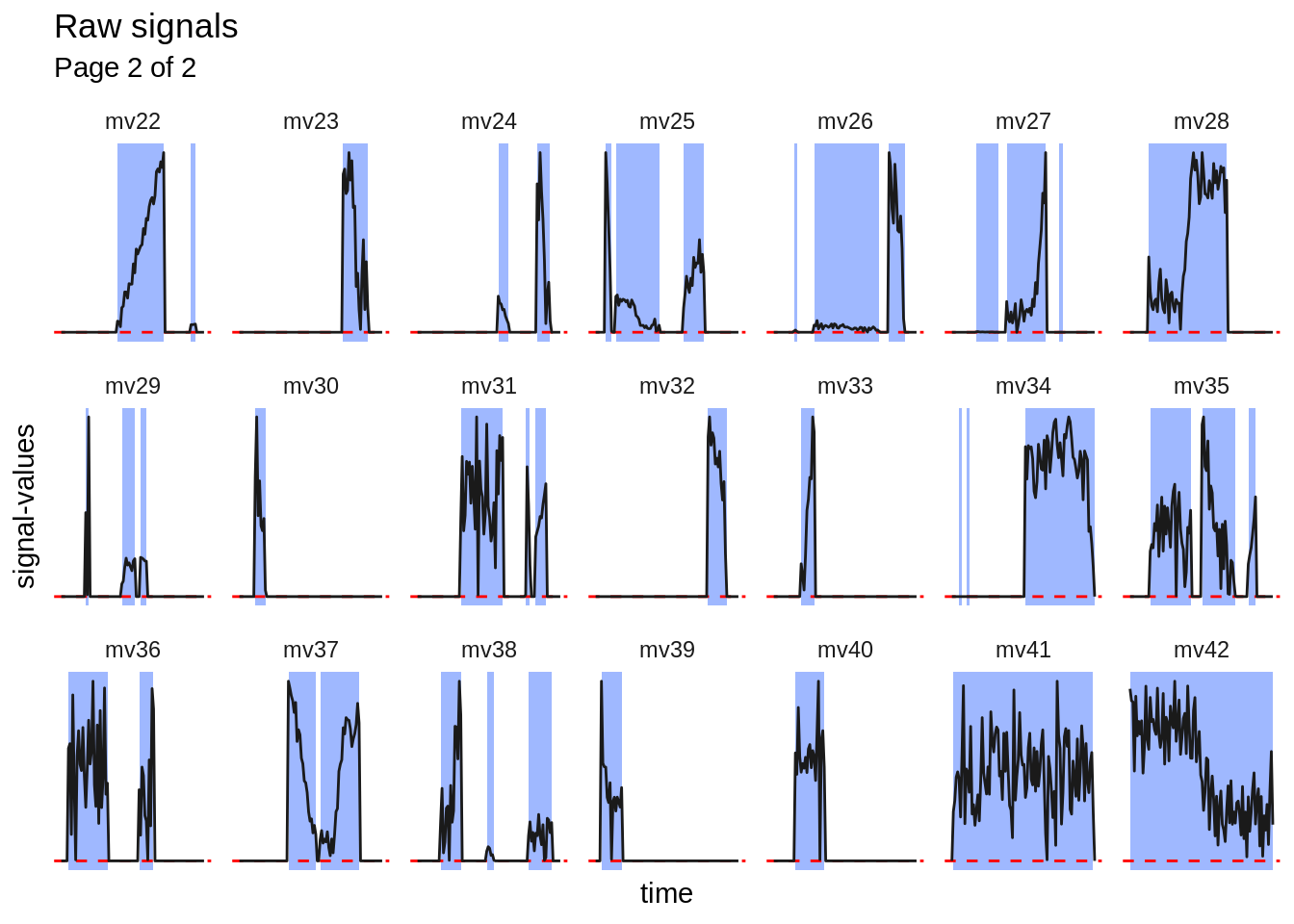

The subsignal-extraction is performed by using mbte_extract_subsignals().

extracted <- mbte_extract_subsignals(nested)
extracted
#> # A tibble: 86 x 3
#>    mv    signal_nr signal           
#>    <chr>     <int> <list>           
#>  1 mv1           1 <tibble [22 × 2]>
#>  2 mv1           2 <tibble [8 × 2]> 
#>  3 mv1           3 <tibble [13 × 2]>
#>  4 mv2           1 <tibble [5 × 2]> 
#>  5 mv3           1 <tibble [20 × 2]>
#>  6 mv3           2 <tibble [22 × 2]>
#>  7 mv4           1 <tibble [3 × 2]> 
#>  8 mv4           2 <tibble [9 × 2]> 
#>  9 mv4           3 <tibble [12 × 2]>
#> 10 mv5           1 <tibble [30 × 2]>
#> # … with 76 more rows

The output shows, that the first signal has been split into three subsignals. The column “signal_nr” has been added to describe the position of the extracted subsignal within the original signal (e.g. signal_nr == 2 indicates, that the corresponding row contains the second subsignal within the orginal signal).

In this example, only subsignals with a length of greater than 11 (arbitrary threshold) are kept. This should ensure, that signals like the one for “mv2” (measurement variable 2) are discarded. Filtering can be done using dplyr. Since signal is a list-column, purrr::map_int() is used to get the number of rows of the corresponding signal (which is stored as a tibble).

NOTE: mbte_reconstruct() should be called, if functions are invoked, which may modify the attributes of the original object (in this case dplyr::filter()).

filtered_dataset <- extracted %>% 
  filter(purrr::map_int(signal, nrow) > 11) %>% 
  mbte_reconstruct(extracted)
filtered_dataset
#> # A tibble: 52 x 3
#>    mv    signal_nr signal           
#>    <chr>     <int> <list>           
#>  1 mv1           1 <tibble [22 × 2]>
#>  2 mv1           3 <tibble [13 × 2]>
#>  3 mv3           1 <tibble [20 × 2]>
#>  4 mv3           2 <tibble [22 × 2]>
#>  5 mv4           3 <tibble [12 × 2]>
#>  6 mv5           1 <tibble [30 × 2]>
#>  7 mv6           1 <tibble [21 × 2]>
#>  8 mv6           3 <tibble [30 × 2]>
#>  9 mv7           1 <tibble [56 × 2]>
#> 10 mv8           1 <tibble [29 × 2]>
#> # … with 42 more rows

Fitting

The remaining rows are analyzed for trends. This is done by fitting an arbitrary model to the subsignals. The only criteria for the used models is, that numeric predictions for the original signal must be computable.

Since the general trend is not always known beforehand, loess() gets used to fit a spline to each subsignal using mbte_fit(). Additonally, a linear model gets fit too.

fitted <- filtered_dataset %>% 
  mbte_fit(
    loess = loess(value ~ t, .signal, span = 0.95),
    lm = lm(value ~ t, .signal)
  )

# resulting table
fitted
#> # A tibble: 52 x 4
#>    mv    signal_nr signal            fits             
#>    <chr>     <int> <list>            <list>           
#>  1 mv1           1 <tibble [22 × 2]> <tibble [22 × 2]>
#>  2 mv1           3 <tibble [13 × 2]> <tibble [13 × 2]>
#>  3 mv3           1 <tibble [20 × 2]> <tibble [20 × 2]>
#>  4 mv3           2 <tibble [22 × 2]> <tibble [22 × 2]>
#>  5 mv4           3 <tibble [12 × 2]> <tibble [12 × 2]>
#>  6 mv5           1 <tibble [30 × 2]> <tibble [30 × 2]>
#>  7 mv6           1 <tibble [21 × 2]> <tibble [21 × 2]>
#>  8 mv6           3 <tibble [30 × 2]> <tibble [30 × 2]>
#>  9 mv7           1 <tibble [56 × 2]> <tibble [56 × 2]>
#> 10 mv8           1 <tibble [29 × 2]> <tibble [29 × 2]>
#> # … with 42 more rows

Users can make use of masked objects for fitting (see documentation of mbte_fit() for details). For example .signal does not exist in the workspace. It gets provided by mbte_fit() to simplify fitting. That way, the user can think of fitting a linear model to a table containing the time- and value-column (in our example named t and value). .signal is just an element of the signal-column of the filtered dataset:

filtered_dataset$signal[[1]] # example element of `.signal`
#> # A tibble: 22 x 2
#>        t value
#>    <int> <dbl>
#>  1    29 36.9 
#>  2    30 22.9 
#>  3    31 21.4 
#>  4    32 31.8 
#>  5    33 21.6 
#>  6    34 27.5 
#>  7    35 22.6 
#>  8    36 19.5 
#>  9    37  7.11
#> 10    38 11.5 
#> # … with 12 more rows

Metric computation

In order to compare the fits, an error metric is computed for each fit. Generally speaking, a trend is present, if the used models are able to generalize the underlying trend of a signal. Therefore, the lower the resulting error metric, the higher the likelyhood for an interesting measurement-parameter worth inversitgating.

For the comparison of the fits, the normalized root mean-squared error is used, since a error metric is required, which is relative to the range of the signal-intensities (signal-values).

nrmse <- function(obs, pred) {
  sqrt(mean((pred - obs)^2)) / (max(obs) - min(obs))
}

metrics <- mbte_compute_metrics(fitted, nrmse = nrmse(.obs, .pred))
metrics
#> # A tibble: 104 x 5
#>    mv    signal_nr fit   metric result
#>    <chr>     <int> <chr> <chr>   <dbl>
#>  1 mv1           1 loess nrmse  0.157 
#>  2 mv1           1 lm    nrmse  0.166 
#>  3 mv1           3 loess nrmse  0.295 
#>  4 mv1           3 lm    nrmse  0.299 
#>  5 mv3           1 loess nrmse  0.243 
#>  6 mv3           1 lm    nrmse  0.252 
#>  7 mv3           2 loess nrmse  0.0872
#>  8 mv3           2 lm    nrmse  0.146 
#>  9 mv4           3 loess nrmse  0.193 
#> 10 mv4           3 lm    nrmse  0.231 
#> # … with 94 more rows

Like for mbte_fit(), mbte_compute_metrics() also uses masking to simplify the metric computation. Here .pred denote the predicted signal-values from the model and .obs are the observed/original values of the signal (both are numeric vectors).

The resulting matrics-table can be filterd accordingly using dplyr. A score gets computed for each signal (identified by the measurement variable and the signal_nr).

NOTE: In this case, calling mbte_reconstruct() is not required, since the result doesen’t have to be of class tbl_mbte, which will only be processed by dplyr and not by the mbte-package directly.

metrics <- metrics %>% 
  group_by(mv, signal_nr) %>% 
  summarize(score = sum(result)) %>% # compute score (lower is better)
  arrange(-desc(score)) %>% # order by result in ascending order
  ungroup() %>% 
  select(mv, signal_nr, score) # only keep relevant columns
metrics
#> # A tibble: 52 x 3
#>    mv    signal_nr  score
#>    <chr>     <int>  <dbl>
#>  1 mv22          1 0.0704
#>  2 mv37          1 0.0965
#>  3 mv21          2 0.102 
#>  4 mv18          2 0.128 
#>  5 mv6           3 0.192 
#>  6 mv15          2 0.206 
#>  7 mv32          1 0.212 
#>  8 mv27          2 0.215 
#>  9 mv10          1 0.217 
#> 10 mv13          1 0.223 
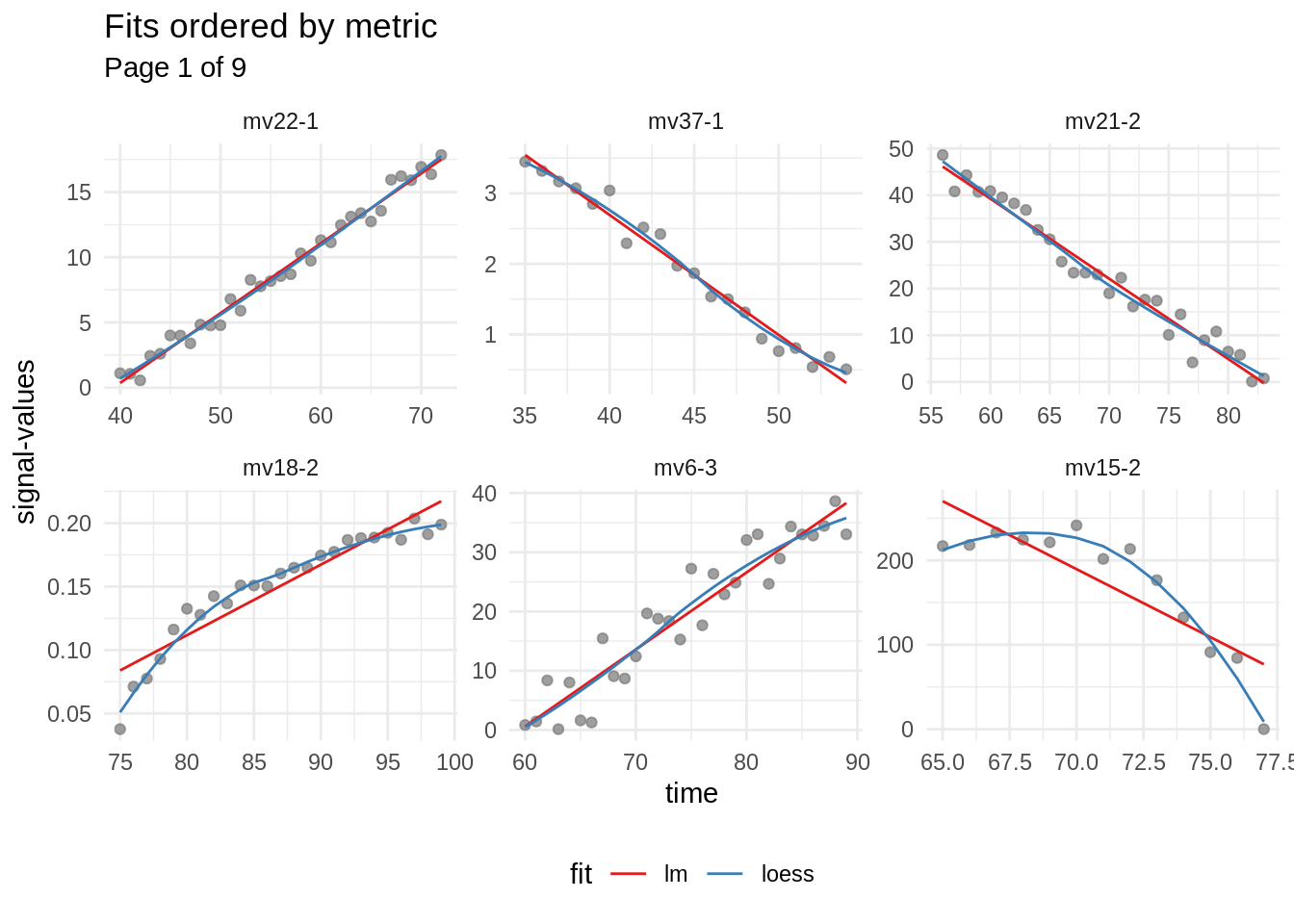
#> # … with 42 more rows

It can be seen, that subsignal nr. 1 of measurement-variable mv22 seems to have the best score. To investigate the fits further, the fitted-table containing the fits is rearranged (order of rows changed according to the best fits). The best-performing fits are put at the beginning of the table.

fitted <- fitted %>% 
  left_join(metrics, by = c("mv", "signal_nr")) %>% # add "score" column
  arrange(-desc(score)) %>% # reorder rows
  select(-score) %>% # remove column "score"
  mbte_reconstruct(fitted)
fitted
#> # A tibble: 52 x 4
#>    mv    signal_nr signal            fits             
#>    <chr>     <int> <list>            <list>           
#>  1 mv22          1 <tibble [33 × 2]> <tibble [33 × 2]>
#>  2 mv37          1 <tibble [20 × 2]> <tibble [20 × 2]>
#>  3 mv21          2 <tibble [28 × 2]> <tibble [28 × 2]>
#>  4 mv18          2 <tibble [25 × 2]> <tibble [25 × 2]>
#>  5 mv6           3 <tibble [30 × 2]> <tibble [30 × 2]>
#>  6 mv15          2 <tibble [13 × 2]> <tibble [13 × 2]>
#>  7 mv32          1 <tibble [14 × 2]> <tibble [14 × 2]>
#>  8 mv27          2 <tibble [28 × 2]> <tibble [28 × 2]>
#>  9 mv10          1 <tibble [25 × 2]> <tibble [25 × 2]>
#> 10 mv13          1 <tibble [72 × 2]> <tibble [72 × 2]>
#> # … with 42 more rows

Visualisation of fits

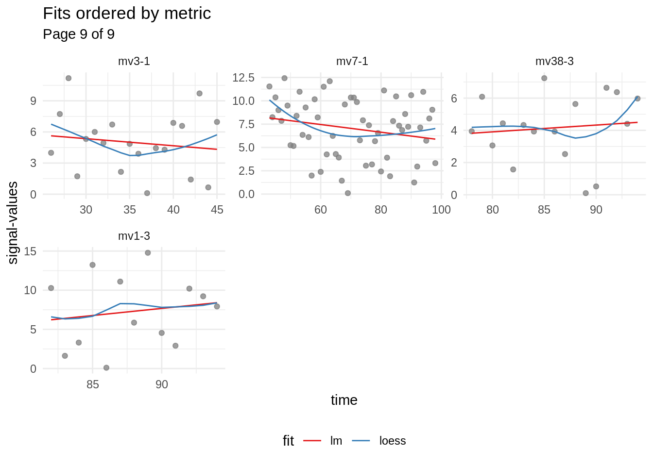
mbte_panel_plot() is used to produce the following visualisations of the fits. Since the fitted-table has been rearranged according to the performance of the corresponding fit, signals containing a clearer trend are drawn first:

fit_vis <- mbte_panel_plot(fitted, {
  ggplot(.u_signals, aes(t, value)) +
    geom_point(alpha = 0.75, color = "grey50") +
    geom_path(aes(color = fit, group = paste0(mv, signal_nr, fit)), .u_fits) +
    scale_color_brewer(palette = "Set1") +
    labs(x = "time", y = "signal-values") +
    ggtitle("Fits ordered by metric", paste("Page", .n_page, "of", .n_pages)) +
    theme_minimal() +
    theme(legend.position = "bottom")
}, mv, signal_nr, nrow = 2, ncol = 3)
fit_vis <- fit_vis[c(1, length(fit_vis))] # only keep best and worst fits

# best fits
fit_vis[[1]]


# worst fits
fit_vis[[2]]

General Workflow

Martin Kerschbaumer

2019-02-19